Circadian soundscape

When dealing with large amounts of audio recordings, visualization plays a key role to evidence the main patterns in the data. In this example we show how to easily combine 96 audio files to build a visual representation of a 24 hour natural soundscape.

Load packages and set variables.

import glob
import matplotlib.pyplot as plt
from maad import sound, util

fpath = '../../data/indices/'  # location of audio files
sample_len = 3  # length in seconds of each audio slice

Build a long list of audio slices of length sample_len.

flist = glob.glob(fpath+'*.wav')
flist.sort()
long_wav = list()
for idx, fname in enumerate(flist):
    s, fs = sound.load(fname)
    s = sound.trim(s, fs, 0, sample_len)
    long_wav.append(s)

Combine all audio recordings applying a crossfade and compute the spectrogram of the resulting mixed audio.

long_wav = util.crossfade_list(long_wav, fs, fade_len=0.5)
Sxx, tn, fn, ext = sound.spectrogram(long_wav, fs,
                                     window='hann', nperseg=1024, noverlap=512)

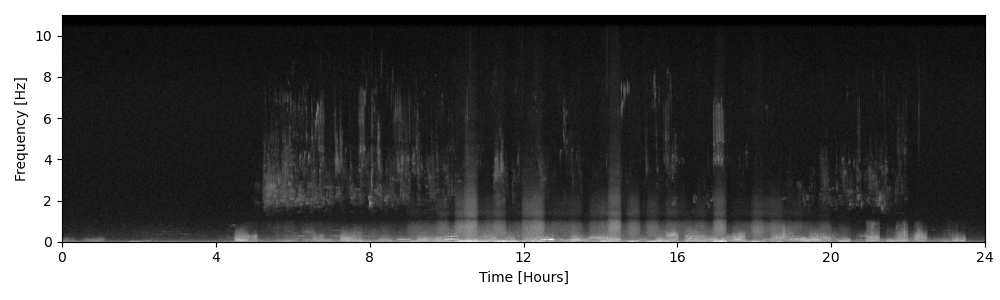
Display the spectrogram. We can see clearly the bird chorus at dawn (5-10 h) and dusk (20-21 h), as well as the wind and airplanes sounds at low frequencies.

fig, ax = plt.subplots(1,1, figsize=(10,3))
util.plot_spectrogram(Sxx, extent=[0, 24, 0, 11],
                      ax=ax, db_range=80, gain=25, colorbar=False)
ax.set_xlabel('Time [Hours]')
ax.set_xticks(range(0,25,4))