Simple audio segmentation

In audio signals, regions of interest are usually regions with high density of energy. The function find_rois_cwt allows finding regions of interest in the signal giving very simple and intuitive parameters: temporal length and frequency limits. This segmentation can be seen as a coarse detection process, the starting point of more advanced classification methods.

The following sound example as two main different soundtypes in the foreground:

• A bouncy trill between 4.5 and 8 kHz lasting approximately 2 seconds.

• A fast descending chirp between 8 and 12 kHz lasting 0.1 approximately seconds.

Load audio file

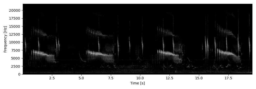
Load an audio file and compute the spectrogram for visualization.

from maad import sound
from maad.rois import find_rois_cwt
from maad.util import plot_spectrogram

s, fs = sound.load('../../data/spinetail.wav')
Sxx, tn, fn, ext = sound.spectrogram(s, fs, nperseg=1024, noverlap=512)
plot_spectrogram(Sxx, extent=ext, db_range=60, gain=20, colorbar=False, figsize=(2.5,10))

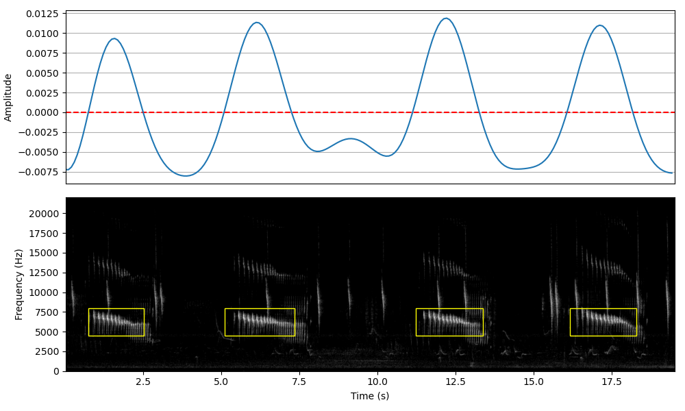
Detect the bouncy trill

The accelerating trill is the song of a small neotropical bird, the Red-faced Spinetail Cranioleuca erythrops. This song can be detected on the recording using the function find_rois_cwt and setting frequency limits flims=(4500,8000) and temporal length of signal tlen=2. The segmentation results are returned as a dataframe with temporal segmentation given by the function and using the frequency limits defined by the user.

df_trill = find_rois_cwt(s, fs, flims=(4500,8000), tlen=2, th=0, display=True, figsize=(10,6))
print(df_trill)

    min_f     min_t   max_f     max_t
0  4500.0   0.74304  8000.0   2.50776
1  4500.0   5.10839  8000.0   7.33751
2  4500.0  11.23846  8000.0  13.37469
3  4500.0  16.16109  8000.0  18.29732

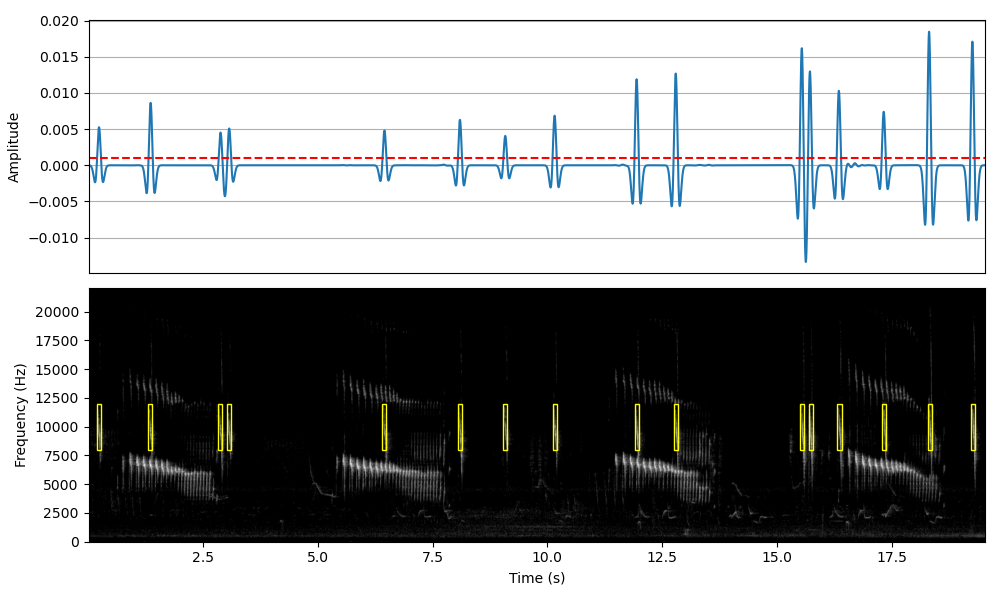
Detect the fast descending chirp

Alternatively, the fast descending chirp (unknown species) can be segmented in the recording by changing the detection parameters, flims and tlen.

df_chirp = find_rois_cwt(s, fs, flims=(8000,12000), tlen=0.1, th=0.001, display=True, figsize=(10,6))
print(df_chirp)

     min_f     min_t    max_f     max_t
0   8000.0   0.18576  12000.0   0.26993
1   8000.0   1.30612  12000.0   1.39900
2   8000.0   2.83574  12000.0   2.91701
3   8000.0   3.02730  12000.0   3.10857
4   8000.0   6.40871  12000.0   6.49288
5   8000.0   8.05152  12000.0   8.14150
6   8000.0   9.04417  12000.0   9.12544
7   8000.0  10.11519  12000.0  10.20517
8   8000.0  11.90023  12000.0  11.99601
9   8000.0  12.75356  12000.0  12.84934
10  8000.0  15.50222  12000.0  15.59220
11  8000.0  15.68508  12000.0  15.77215
12  8000.0  16.31202  12000.0  16.40490
13  8000.0  17.29016  12000.0  17.38014
14  8000.0  18.27701  12000.0  18.37279
15  8000.0  19.22032  12000.0  19.31610