Template matching

Template matching is a simple but powerfull method to detect a stereotyped sound of interest using a template signal. This example shows how to use the normalized cross-correlation of spectrograms. For a more detailed information on how to implement this technique in a large dataset check references [1,2].

References

[1]

Ulloa, Juan Sebastian, Amandine Gasc, Phillipe Gaucher, Thierry Aubin, Maxime Réjou-Méchain, and Jérôme Sueur. 2016. “Screening Large Audio Datasets to Determine the Time and Space Distribution of Screaming Piha Birds in a Tropical Forest.” Ecological Informatics 31:91–99. doi: 10.1016/j.ecoinf.2015.11.012.

[2]

Brunelli, Roberto. 2009. Template Matching Techniques in Computer Vision: Theory and Practice. John Wiley and Sons, Ltd.

Load required modules

import matplotlib.pyplot as plt
from maad import sound, util
from maad.rois import template_matching

Compute spectrograms

The first step is to compute the spectrogram of the template and the target audio. It is important to use the same spectrogram parameters for both signals in order to get adecuate results. For simplicity, we will take the template from the same target audio signal, but the template can be loaded from another file.

# Set spectrogram parameters
tlims = (9.8, 10.5)
flims = (6000, 12000)
nperseg = 1024
noverlap = 512
window = 'hann'
db_range = 80

# load data
s, fs = sound.load('../../data/spinetail.wav')

# Compute spectrogram for template signal
Sxx_template, _, _, _ = sound.spectrogram(s, fs, window, nperseg, noverlap, flims, tlims)
Sxx_template = util.power2dB(Sxx_template, db_range)

# Compute spectrogram for target audio
Sxx_audio, tn, fn, ext = sound.spectrogram(s, fs, window, nperseg, noverlap, flims)
Sxx_audio = util.power2dB(Sxx_audio, db_range)

Compute the cross-correlation of spectrograms

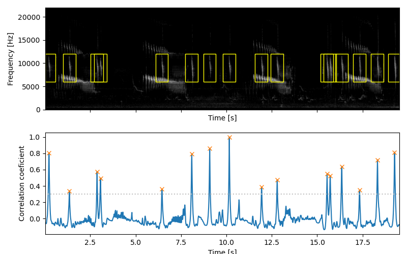
Compute the cross-correlation of spectrograms and find peaks in the resulting signal using the template matching function. The template_matching functions gives temporal information on the location of the audio and frequency limits must be added.

peak_th = 0.3 # set the threshold to find peaks
xcorrcoef, rois = template_matching(Sxx_audio, Sxx_template, tn, ext, peak_th)
rois['min_f'] = flims[0]
rois['max_f'] = flims[1]
print(rois)

    peak_time  xcorrcoef      min_t      max_t  min_f  max_f
0    0.220590   0.806825   0.011610   0.568889   6000  12000
1    1.346757   0.340795   0.998458   1.695057   6000  12000
2    2.867664   0.573861   2.519365   3.215964   6000  12000
3    3.065034   0.494980   2.716735   3.413333   6000  12000
4    6.443537   0.363005   6.095238   6.791837   6000  12000
5    8.092154   0.795268   7.743855   8.440454   6000  12000
6    9.079002   0.859184   8.730703   9.427302   6000  12000
7   10.158730   1.000000   9.810431  10.507029   6000  12000
8   11.935057   0.385691  11.586757  12.283356   6000  12000
9   12.794195   0.475053  12.445896  13.142494   6000  12000
10  15.545760   0.546829  15.197460  15.894059   6000  12000
11  15.719909   0.523297  15.371610  16.068209   6000  12000
12  16.358458   0.639122  16.010159  16.706757   6000  12000
13  17.333696   0.347990  16.985397  17.681995   6000  12000
14  18.320544   0.720789  17.972245  18.668844   6000  12000
15  19.260952   0.813835  18.912653  19.527982   6000  12000

Plot results

Finally, you can plot the detection results or save them as a csv file.

Sxx, tn, fn, ext = sound.spectrogram(s, fs, window, nperseg, noverlap)
fig, ax = plt.subplots(2,1, figsize=(8, 5), sharex=True)
util.plot_spectrogram(Sxx, ext, db_range=80, ax=ax[0], colorbar=False)
util.overlay_rois(Sxx, util.format_features(rois, tn, fn), fig=fig, ax=ax[0])
ax[1].plot(tn[0: xcorrcoef.shape[0]], xcorrcoef)
ax[1].hlines(peak_th, 0, tn[-1], linestyle='dotted', color='0.75')
ax[1].plot(rois.peak_time, rois.xcorrcoef, 'x')
ax[1].set_xlabel('Time [s]')
ax[1].set_ylabel('Correlation coeficient')
plt.show()