Detection distance estimation

When sound travels in air (or in water), initial acoustic signature may change regarding distances due to attenuation. Sound attenuation in natural environment is very complex to model. We propose to reduce the complexity by decomposing the sound attenuation to three main sources of attenuation : - the geometric attenuation (Ageo) also known as spreading loss or geometric dispersion, - the atmospheric attenuation (Aatm) - and the habitat attenuation (Ahab). The later encompasses several sources of attenuation and might be seen as a proxy.

Knowing the attenuation law and the sound level at each frequency, it is possible to estimate the detection distance of each frequency component of that sound

In this example, we will estimate the detection distance of each frequency component of a sound that travels in rainforest at noon, when the ambient sound level is the lowest.

# import numpy
import numpy as np
# import the graphic library
import matplotlib.pyplot as plt
plt.style.use('ggplot')
# import maad
from maad import sound, spl, util

Let’s decide that the propagation sound is a wideband sound ranging from 0Hz to 20000Hz with an initial sound pressure level of 80 dBSPL at 1m which corresponds to the sum of the sound pressure level along the full frequency bandwidth. So we need first to spread the intial sound pressure level over this frequency bandwidth.

# frequency vector from 0Hz to 20000Hz, with 1000Hz resolution
f = np.arange(0,20000,1000)
# Repartition of the initial sound pressure level along each frequency bin
L0 = 80
L0_per_bin = spl.dBSPL_per_bin(L0,f)
print(L0_per_bin)
# Distance in m at which the initial sound pressure level is measured
r0 = 1

[66.98970004 66.98970004 66.98970004 66.98970004 66.98970004 66.98970004
 66.98970004 66.98970004 66.98970004 66.98970004 66.98970004 66.98970004
 66.98970004 66.98970004 66.98970004 66.98970004 66.98970004 66.98970004
 66.98970004 66.98970004]

The detection distance is mostly driven by the sound pressure level of the background noise (or ambient sound). Let’s define an array with the sound pressure level experimentaly measured in a rainforest (French Guiana) at noon for each frequency bin (from 0Hz to 20kHz).

L_bkg = np.array([44.270917, 27.586848, 25.60843 , 23.205826, 20.631086, 24.080126,
                  19.032034, 33.455814, 44.420644, 19.751421, 11.932672,  9.641225,
                  8.075566,  7.447614,  6.991958,  7.854252, 11.911974,  4.192154,
                  3.234791,  2.936258])

We know the initial sound pressure level LO at the distance r0 = 1m as well as the sound pressure level of the background L_bkg, then it is possible to estimate the detection distance for each frequency bin. We set the temperature at 24°C and the relative humidity at 87% as there are common values for rainforest. We also set the coefficient of attenuation of the habitat to 0.02dB/kHz/m which is also representative of the attenuation of rainforest habitat.

f, r = spl.detection_distance (L_bkg, L0_per_bin, f, r0, t = 24, rh = 87, a0=0.02)

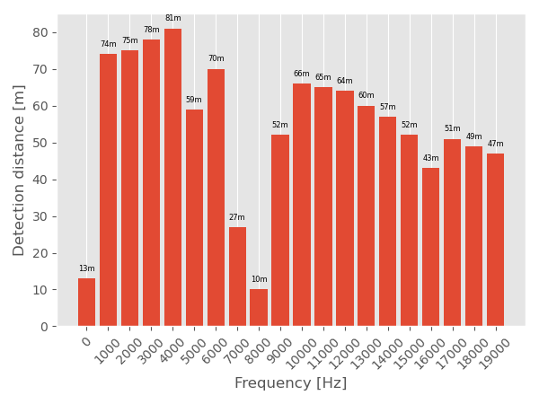
Display the detection distance for each frequency as a bar plot. We can observe that the detection distance is highly variable from 10m at 8kHz till 81m for 4kHz. The low detection distance between 7kHz to 8kHz is due to the stridulations of the insects that is very loud. It masks the propagation of the audio signal at a very short distance.

# Define a function to add value labels
def valuelabel(f,r):
    for i in range(len(f)):
        plt.text(i,
                 r[i]+2,
                 '%dm' % r[i],
                 ha = 'center',
                 size=6,
                )

# Create the figure and set the size
fig = plt.figure()
fig.set_figwidth(6)
fig.set_figheight(4.5)

# Create bars
y_pos = np.arange(len(f))
plt.bar(y_pos, r)

# Create names on the x-axis
plt.xticks(y_pos, f)
plt.xticks(rotation=45)

# Call function
valuelabel(f, r)

# Define labels
plt.ylabel("Detection distance [m]")
plt.xlabel("Frequency [Hz]")

# Show graphic
plt.tight_layout()
plt.grid(axis='y')
plt.show()