Audio representation

An audio signal can be represented in both, temporal and spectral domains. These representations are complementary and fundamental to understand the audio signal characteristics. In this introductory example we will load an audio signal, apply basic transformations to better understand its features in time and frequency.

Load an audio file and plot the waveform

import matplotlib.pyplot as plt
from maad import sound
from maad import util

s, fs = sound.load('../../data/spinetail.wav')
util.plot_wave(s, fs)
plt.show()

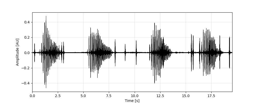
It can be noticed that in this audio there are four consecutive songs of the spinetail Cranioleuca erythorps, every song lasting of approximatelly two seconds. Let’s trim the signal to zoom in on the details of the song.

s_trim = sound.trim(s, fs, 5, 8)

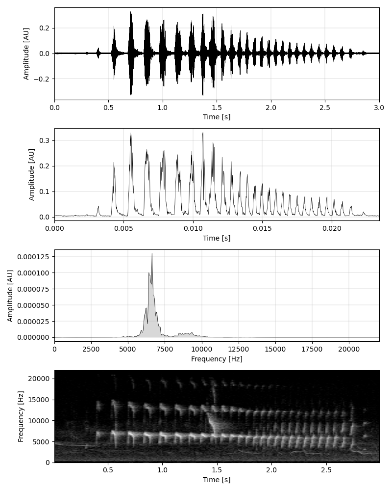
Onced trimmed, lets compute the envelope of the signal, the Fourier and short-time Fourier transforms.

env = sound.envelope(s_trim, mode='fast', Nt=128)
pxx, fidx = sound.spectrum(s, fs, nperseg=1024, method='welch')
Sxx, tn, fn, ext = sound.spectrogram(s_trim, fs, window='hann', nperseg=1024, noverlap=512)

Finally, we can visualize the signal characteristics in the temporal and spectral domains.

fig, ax = plt.subplots(4,1, figsize=(8,10))
util.plot_wave(s_trim, fs, ax=ax[0])
util.plot_wave(env, fs, ax=ax[1])
util.plot_spectrum(pxx, fidx, ax=ax[2])
util.plot_spectrogram(Sxx, extent=ext, ax=ax[3], colorbar=False)
plt.show()