Download metadata from Xeno-Canto to infer species activities¶

The goal of this example is to show how to download metadata from Xeno-Canto to infer species activities. We focus on the activity of european woodpeckers.

Dependencies: To execute this example you need to have installed pandas package.

(from https://woodpeckersofeurope.blogspot.com/2007/11/drumming.html) Woodpeckers of Europe 10 species of woodpecker (Picidae) breed in Europe: 9 resident species and the migratory Wryneck. 8 of these 10 also occur outside Europe, with the distribution of Eurasian Three-toed, White-backed, Lesser Spotted, Great Spotted, Black & Grey-headed Woodpeckers stretching eastwards from the Western Palearctic into Asia, whilst Syrian is found in the Middle East & Asia Minor & Wryneck winters in Africa. The global ranges of Green & Middle Spotted Woodpeckers are confined to the Western Palearctic.

Eurasian Three-toed : Picoides tridactylus White-backed : Dendrocopos leucotos Lesser Spotted : Dryobates minor Great Spotted : Dendrocopos major Black : Dryocopus martius Grey-headed : Picus canus Syrian : Dendrocopos syriacus Wryneck : Jynx torquilla Green : Picus viridis Middle Spotted : Dendrocoptes medius

# sphinx_gallery_thumbnail_path = './_images/sphx_glr_plot_woodpeckers_drumming_annual_activity.png'

import pandas as pd
import matplotlib.pyplot as plt
import numpy as np

from maad import util

Query Xeno-Canto¶

array with english name and scientific name of all european woodpeckers

data = [['Eurasian Three-toed', 'Picoides tridactylus'],
        ['White-backed',        'Dendrocopos leucotos'],
        ['Lesser Spotted',          'Dryobates minor'],
        ['Great Spotted',       'Dendrocopos major'],
        ['Black',                   'Dryocopus martius'],
        ['Grey-headed',             'Picus canus'],
        ['Syrian',              'Dendrocopos syriacus'],
        ['Wryneck',             'Jynx torquilla'],
        ['Green',               'Picus viridis'],
        ['Middle Spotted',      'Dendrocoptes medius']]

creation of a dataframe for the array with species names

df_species = pd.DataFrame(data,columns =['english name',
                                         'scientific name'])

get the genus and species needed for Xeno-Canto

gen = []
sp = []
for name in df_species['scientific name']:
    gen.append(name.rpartition(' ')[0])
    sp.append(name.rpartition(' ')[2])

Build the query dataframe with columns paramXXX gen : genus cnt : country area : continent (europe, america, asia, africa) q : quality (q_gt => quality equal or greater than) len : length of the audio file (len_lt => length lower than;

len_gt => length greater than )

type : type of sound : ‘song’ or ‘call’ or ‘drumming’ Please have a look here to know all the parameters and how to use them : https://xeno-canto.org/help/search

df_query = pd.DataFrame()
df_query['param1'] = gen
df_query['param2'] = sp
df_query['param4'] ='type:drumming'
df_query['param5'] ='area:europe'

Get recordings metadata corresponding to the query

df_dataset = util.xc_multi_query(df_query,
                                 format_time = True,
                                 format_date = True,
                                 verbose=True)

Out:

Loading page 1...
https://www.xeno-canto.org/api/2/recordings?query=Picoides%20tridactylus%20area:europe&page=1
searchTerms ['Picoides', 'tridactylus', 'area:europe']
Keeped metadata for 189 files after formating time
Keeped metadata for 125 files after formating date
Found 1 pages in total.
Saved metadata for 125 files
Loading page 1...
https://www.xeno-canto.org/api/2/recordings?query=Dendrocopos%20leucotos%20area:europe&page=1
searchTerms ['Dendrocopos', 'leucotos', 'area:europe']
Keeped metadata for 138 files after formating time
Keeped metadata for 103 files after formating date
Found 1 pages in total.
Saved metadata for 103 files
Loading page 1...
https://www.xeno-canto.org/api/2/recordings?query=Dryobates%20minor%20area:europe&page=1
Loading page 2...
https://www.xeno-canto.org/api/2/recordings?query=Dryobates%20minor%20area:europe&page=2
searchTerms ['Dryobates', 'minor', 'area:europe']
Keeped metadata for 385 files after formating time
Keeped metadata for 296 files after formating date
Found 2 pages in total.
Saved metadata for 296 files
Loading page 1...
https://www.xeno-canto.org/api/2/recordings?query=Dendrocopos%20major%20area:europe&page=1
Loading page 2...
https://www.xeno-canto.org/api/2/recordings?query=Dendrocopos%20major%20area:europe&page=2
Loading page 3...
https://www.xeno-canto.org/api/2/recordings?query=Dendrocopos%20major%20area:europe&page=3
Loading page 4...
https://www.xeno-canto.org/api/2/recordings?query=Dendrocopos%20major%20area:europe&page=4
Loading page 5...
https://www.xeno-canto.org/api/2/recordings?query=Dendrocopos%20major%20area:europe&page=5
searchTerms ['Dendrocopos', 'major', 'area:europe']
Keeped metadata for 653 files after formating time
Keeped metadata for 483 files after formating date
Found 5 pages in total.
Saved metadata for 483 files
Loading page 1...
https://www.xeno-canto.org/api/2/recordings?query=Dryocopus%20martius%20area:europe&page=1
Loading page 2...
https://www.xeno-canto.org/api/2/recordings?query=Dryocopus%20martius%20area:europe&page=2
Loading page 3...
https://www.xeno-canto.org/api/2/recordings?query=Dryocopus%20martius%20area:europe&page=3
searchTerms ['Dryocopus', 'martius', 'area:europe']
Keeped metadata for 263 files after formating time
Keeped metadata for 198 files after formating date
Found 3 pages in total.
Saved metadata for 198 files
Loading page 1...
https://www.xeno-canto.org/api/2/recordings?query=Picus%20canus%20area:europe&page=1
Loading page 2...
https://www.xeno-canto.org/api/2/recordings?query=Picus%20canus%20area:europe&page=2
searchTerms ['Picus', 'canus', 'area:europe']
Keeped metadata for 79 files after formating time
Keeped metadata for 58 files after formating date
Found 2 pages in total.
Saved metadata for 58 files
Loading page 1...
https://www.xeno-canto.org/api/2/recordings?query=Dendrocopos%20syriacus%20area:europe&page=1
searchTerms ['Dendrocopos', 'syriacus', 'area:europe']
/Volumes/lacie_macosx/github/scikit-maad/maad/util/xeno_canto.py:144: SettingWithCopyWarning:
A value is trying to be set on a copy of a slice from a DataFrame

See the caveats in the documentation: https://pandas.pydata.org/pandas-docs/stable/user_guide/indexing.html#returning-a-view-versus-a-copy
  df_dataset['time'][df_dataset.time.str.match('^([0-9])[:]([0-5][0-9])$')] = '0' + df_dataset[df_dataset.time.str.match('^([0-9])[:]([0-5][0-9])$')].time
Keeped metadata for 22 files after formating time
Keeped metadata for 18 files after formating date
Found 1 pages in total.
Saved metadata for 18 files
Loading page 1...
https://www.xeno-canto.org/api/2/recordings?query=Jynx%20torquilla%20area:europe&page=1
Loading page 2...
https://www.xeno-canto.org/api/2/recordings?query=Jynx%20torquilla%20area:europe&page=2
searchTerms ['Jynx', 'torquilla', 'area:europe']
Keeped metadata for 0 files after formating time
Keeped metadata for 0 files after formating date
Found 2 pages in total.
Saved metadata for 0 files
Loading page 1...
https://www.xeno-canto.org/api/2/recordings?query=Picus%20viridis%20area:europe&page=1
Loading page 2...
https://www.xeno-canto.org/api/2/recordings?query=Picus%20viridis%20area:europe&page=2
searchTerms ['Picus', 'viridis', 'area:europe']
Keeped metadata for 32 files after formating time
Keeped metadata for 19 files after formating date
Found 2 pages in total.
Saved metadata for 19 files
Loading page 1...
https://www.xeno-canto.org/api/2/recordings?query=Dendrocoptes%20medius%20area:europe&page=1
Loading page 2...
https://www.xeno-canto.org/api/2/recordings?query=Dendrocoptes%20medius%20area:europe&page=2
searchTerms ['Dendrocoptes', 'medius', 'area:europe']
Keeped metadata for 22 files after formating time
Keeped metadata for 17 files after formating date
Found 2 pages in total.
Saved metadata for 17 files

Creation of a dataframe with the number of files per species per 30mins¶

Using the metadata collected from Xeno-Canto, we create a new dataframe containing the number of files per species and per time slot (30 mins). The goal is to create a dataframe with diel pattern of activity for all species with a time resolution of 30 mins.

# make a copy of the dataset to avoid any modification of the original dataset
df = df_dataset.copy()
# remove all rows where data is missing (NA)
df.dropna(subset=['time'], inplace=True)
# Convert time into datetime
df['time'] = pd.to_datetime(df['time'], format="%H:%M")

New dataframe with the number of audio files per time slot. The period of the time slot is 30 min

df_count = pd.DataFrame()
list_species = df['en'].unique()
for species in list_species :
    df_temp = pd.DataFrame()
    df_temp['count'] = df[df['en']==species].set_index(['time']).resample('30T').count().iloc[:,0]
    df_temp['species'] = species
    df_count = df_count.append(df_temp)

# create a column with time only
df_count['time'] = df_count.index.strftime('%H:%M')

Creation of a dataframe with the number of files per species per week¶

Using the metadata collected from Xeno-Cant, we create a new dataframe containing the number of files per species and per week. The goal is to create a dataframe with annual pattern of activity for all species with a week (7 days) resolution.

# make a copy of the dataset to avoid any modification of the original dataset
df = df_dataset.copy()
# remove all rows where data is missing (NA)
df.dropna(subset=['week'], inplace=True)

New dataframe with the number of audio files per week

df_week_count = pd.DataFrame()
list_species = df['en'].unique()
for species in list_species :
    df_temp = pd.DataFrame()
    df_temp['count'] = df[df['en']==species].set_index(['week']).index.value_counts()
    df_temp['species'] = species
    df_week_count = df_week_count.append(df_temp)

# create a column with time only
df_week_count["week"] = df_week_count.index

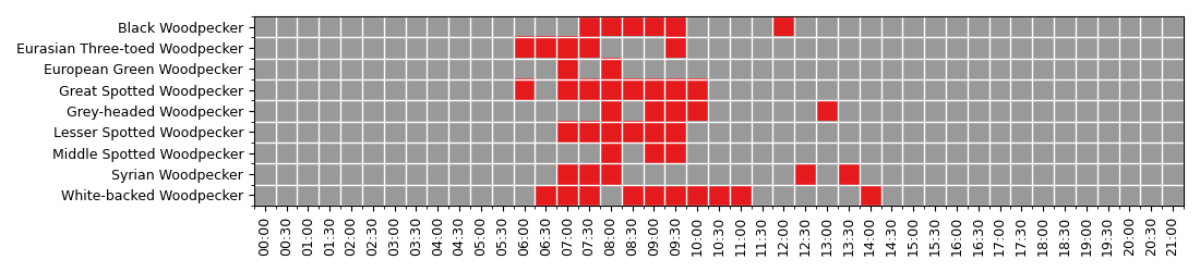
Display a heatmap of diel activity¶

make a copy of the dataset to avoid any modification of the original dataset

df = df_count.copy()

find the number of counts that corresponds to 50% of the counts

for species in list_species:
    # find the threshold value
    count_50_threshold = df[df_count['species']==species]['count'].sum()*(0.50)
    # extract the counting value of the category
    aa = df[df_count['species']==species]['count'].values
    # sort the counts (ascending)
    aa.sort()
    # reverse the order (descending)
    aa = aa[::-1]
    # find the index where the cumulative sum of the count is higher
    idx = np.where(aa.cumsum() >= count_50_threshold)[0]
    aa[idx[0]]
    df.loc[(df_count['species'] == species) & (df['count']< aa[idx[0]]), 'count'] = 0
    df.loc[(df_count['species'] == species) & (df['count']>=aa[idx[0]]), 'count'] = 1

Display the heatmap to see when (time of the day) the woodpeckers are active. Woodpeckers are the most active during the morning, between 6:00am till 10:00am.

df = df.pivot( 'species', 'time', "count")
df = df.fillna(0)

# plot figure
fig = plt.figure(figsize= (11,2.5))
ax = fig.add_subplot(111)
ax.imshow(df, aspect="auto", interpolation="None", cmap="Set1_r")

# Major ticks
ax.set_xticks(np.arange(0, len(list(df)), 1))
ax.set_yticks(np.arange(0, len(df.index), 1))

# Labels for major ticks
ax.set_xticklabels(list(df),
                   fontsize=9,
                   rotation=90)
ax.set_yticklabels(df.index,
                   fontsize=9)

# Minor ticks
ax.set_xticks(np.arange(-0.5, len(list(df)), 1), minor=True)
ax.set_yticks(np.arange(-0.5, len(df.index), 1), minor=True)

# Gridlines based on minor ticks
ax.grid(which='major', color='w', linestyle='-', linewidth=0)
ax.grid(which='minor', color='w', linestyle='-', linewidth=1)

fig.tight_layout()

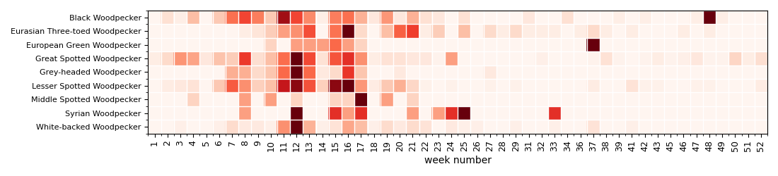
Display a heatmap of annual activity with week resolution¶

make a copy of the dataset to avoid any modification of the original dataset

df = df_week_count.copy()

create a new dataframe with the normalized number of audio files per week

for species in list_species:
    df.loc[df['species'] == species, 'count'] = (df[df['species'] == species]['count']
                                                 /
                                                 np.max(df[df['species'] == species]['count']))

Display the heatmap to see when (annually) the woodpeckers are active. Woodpeckers are the most active during the winter and beginning of spring (Februrary to April).

df = df.pivot( 'species', 'week', "count")
df = df.fillna(0)

# plot figure
fig = plt.figure(figsize= (11,2.5))
ax = fig.add_subplot(111)

ax.imshow(df, aspect="auto", interpolation="None", cmap="Reds")

# Major ticks
ax.set_xticks(np.arange(0, len(list(df)), 1))
ax.set_yticks(np.arange(0, len(df.index), 1))

# Labels for major ticks
ax.set_xticklabels(list(df),
                   fontsize=9,
                   rotation=90)
ax.set_yticklabels(df.index,
                   fontsize=8)

# Minor ticks
ax.set_xticks(np.arange(-0.5, len(list(df)), 1), minor=True)
ax.set_yticks(np.arange(-0.5, len(df.index), 1), minor=True)

# Gridlines based on minor ticks
ax.grid(which='major', color='w', linestyle='-', linewidth=0)
ax.grid(which='minor', color='w', linestyle='-', linewidth=1)

# add the title of the x-axis
ax.set_xlabel("week number")

fig.tight_layout()

Total running time of the script: ( 1 minutes 35.701 seconds)

Gallery generated by Sphinx-Gallery