Find Regions of interest (ROIs) in a spectrogram

A spectrogram is a time-frequency (2d) representation of a audio recording. Each acoustic event nested in the audio recording is represented by an acoustic signature. When sounds does not overlap in time and frequency, it is possible to extract automatically the acoustic signature as a region of interest (ROI) by different image processing tools such as binarization, double thresholding, mathematical morphology tools…

Dependencies: To execute this example you will need to have installed the scikit-image, scikit-learn and pandas Python packages.

# sphinx_gallery_thumbnail_path = './_images/sphx_glr_plot_compare_auto_and_manual_rois_selection_005.png'

Load required modules

import numpy as np
import pandas as pd
from sklearn.cluster import KMeans
from sklearn.preprocessing import StandardScaler
from maad import sound, rois, features
from maad.util import (
   power2dB, plot2d, format_features, read_audacity_annot,
   overlay_rois, overlay_centroid
   )

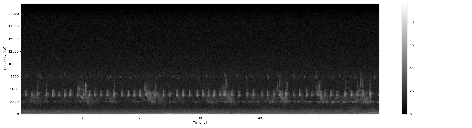
First, load and audio file and compute the power spectrogram.

s, fs = sound.load('../../data/cold_forest_daylight.wav')

dB_max = 96

Sxx_power, tn, fn, ext = sound.spectrogram(
   x=s,
   fs=fs,
   nperseg=1024,
   noverlap=1024//2
   )

# Convert the power spectrogram into dB, add dB_max which is the maximum decibel
# range when quantification bit is 16bits and display the result
Sxx_db = power2dB(Sxx_power) + dB_max

plot2d(
   im=Sxx_db,
   **{
      'vmin':0,
      'vmax':dB_max,
      'extent':ext
      }
   )

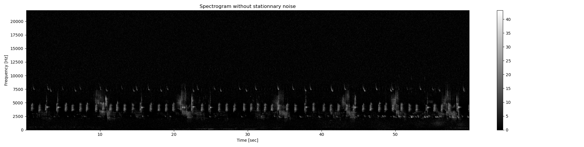
Then, relevant acoustic events are extracted directly from the power spectrogram based on a double thresholding technique. The result is binary image called a mask. Double thresholding technique is more sophisticated than basic thresholding based on a single value. First, a threshold selects pixels with high value (i.e. high acoustic energy). They should belong to an acoustic event. They are called seeds. From these seeds, we aggregate pixels connected to the seed with value higher than the second threslhold. These new pixels become seed and the aggregating process continue until no more new pixels are aggregated, meaning that there is no more connected pixels with value upper than the second threshold value.

# First we remove the stationary background in order to increase the contrast [1]
# Then we convert the spectrogram into dB
Sxx_power_noNoise= sound.median_equalizer(
   Sxx=Sxx_power,
   display=True,
   **{'extent':ext}
   )
Sxx_db_noNoise = power2dB(Sxx_power_noNoise)

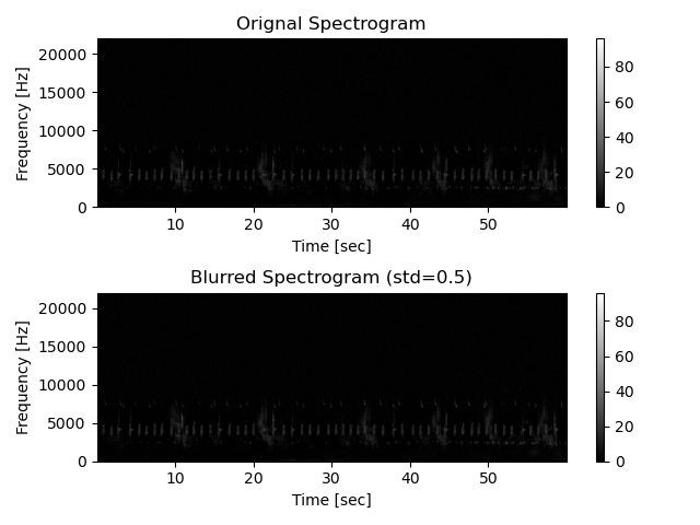
# Then we smooth the spectrogram in order to facilitate the creation of masks as
# small sparse details are merged if they are close to each other
Sxx_db_noNoise_smooth = sound.smooth(
   Sxx=Sxx_db_noNoise,
   std=0.5,
   display=True,
   savefig=None,
   **{
      'vmin':0,
      'vmax':dB_max,
      'extent':ext
      }
   )

# Then we create a mask (i.e. binarization of the spectrogram) by using the
# double thresholding technique
im_mask = rois.create_mask(
   im=Sxx_db_noNoise_smooth,
   mode_bin='relative',
   bin_std=8,
   bin_per=0.5,
   verbose=False,
   display=False
   )

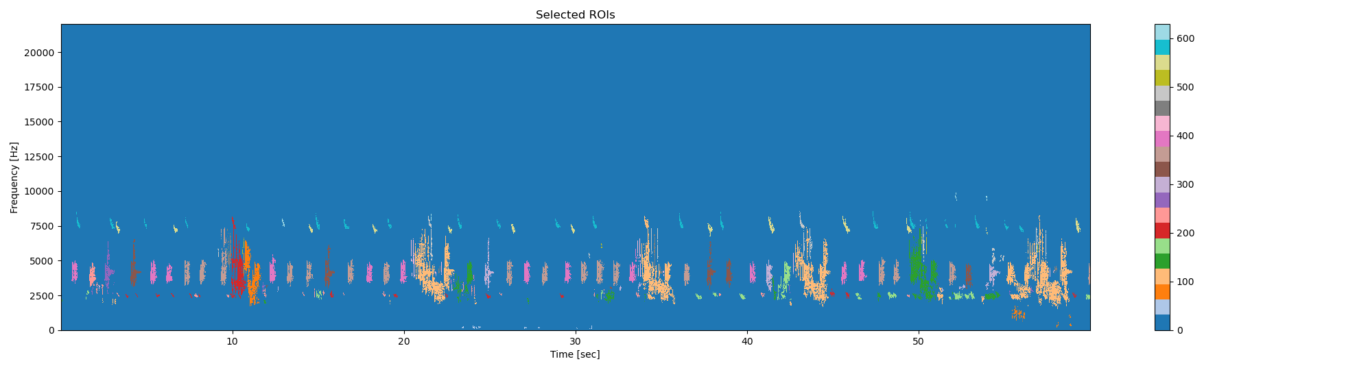
# Finaly, we put together pixels that belong to the same acoustic event, and
# remove very small events (<=25 pixel²)
im_rois, df_rois = rois.select_rois(
   im_bin=im_mask,
   min_roi=25,
   max_roi=None,
   display= True,
   **{'extent':ext}
   )

# format dataframe df_rois in order to convert pixels into time and frequency
df_rois = format_features(
   df=df_rois,
   tn=tn,
   fn=fn
   )

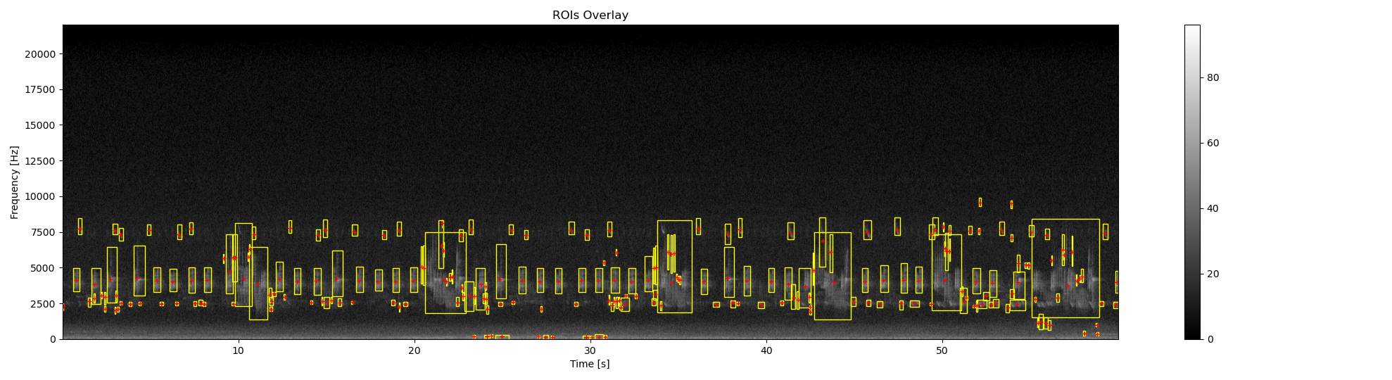
# overlay bounding box on the original spectrogram
ax0, fig0 = overlay_rois(
   im_ref=Sxx_db,
   rois=df_rois,
   **{
      'vmin':0,
      'vmax':dB_max,
      'extent':ext
      }
   )

# Compute centroids
df_centroid = features.centroid_features(
   Sxx=Sxx_db,
   rois=df_rois,
   im_rois=im_rois
   )

# format dataframe df_centroid in order to convert pixels into time and frequency
df_centroid = format_features(
   df=df_centroid,
   tn=tn,
   fn=fn
   )

# overlay centroids on the original spectrogram
ax0, fig0 = overlay_centroid(
   im_ref=Sxx_db,
   centroid=df_centroid,
   savefig=None,
   **{
      'vmin':0,
      'vmax':dB_max,
      'extent':ext,
      'ms':4,
      'marker':'+',
      'color':'red',
      'fig':fig0,
      'ax':ax0
      }
   )

• 
• 
• 
• 

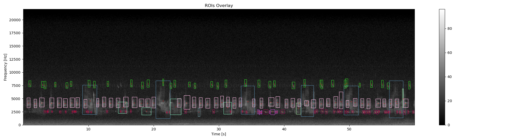
Let’s compare with the manual annotation (Ground Truth GT) obtained with Audacity software. Each acoustic signature is manually selected and labeled. All similar acoustic signatures are labeled with the same name

df_rois_GT = read_audacity_annot('../../data/cold_forest_daylight_label.txt')  ## annotations using Audacity

# drop rows with frequency and time outside of tn and fn
df_rois_GT = df_rois_GT[(df_rois_GT.min_t >= tn.min()) &
                        (df_rois_GT.max_t <= tn.max()) &
                        (df_rois_GT.min_f >= fn.min()) &
                        (df_rois_GT.max_f <= fn.max())]

# format dataframe df_rois in order to convert time and frequency into pixels
df_rois_GT = format_features(df_rois_GT, tn, fn)

# overlay bounding box on the original spectrogram
ax1, fig1 = overlay_rois(
   im_ref=Sxx_db,
   rois=df_rois_GT,
   **{
      'vmin':0,
      'vmax':dB_max,
      'extent':ext
      }
   )

# Compute centroids
df_centroid_GT = features.centroid_features(
   Sxx=Sxx_db,
   rois=df_rois_GT
   )

# format dataframe df_centroid_GT in order to convert pixels into time and frequency
df_centroid_GT = format_features(
   df=df_centroid_GT,
   tn=tn,
   fn=fn
   )

# overlay centroids on the original spectrogram
ax1, fig1 = overlay_centroid(
   im_ref=Sxx_db,
   centroid=df_centroid_GT,
   savefig=None,
   **{
      'vmin':0,
      'vmax':dB_max,
      'extent':ext,
      'ms':2,
      'marker':'+',
      'color':'red',
      'fig':fig1,
      'ax':ax1
      }
   )

# print informations about the rois
print ('Total number of ROIs : %2.0f' %len(df_rois_GT))
print ('Number of different ROIs : %2.0f' %len(np.unique(df_rois_GT['label'])))

Total number of ROIs : 159
Number of different ROIs :  8

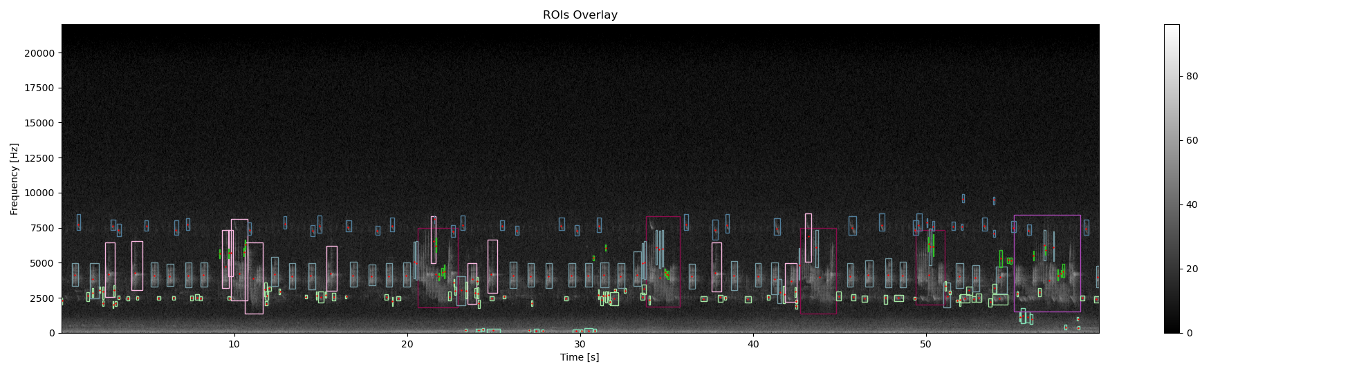
Now we cluster the ROIS depending on 3 ROIS features : - centroid_f : frequency position of the roi centroid - duration_t : duration of the roi - bandwidth_f : frequency bandwidth of the roi The clustering is done by the so-called KMeans clustering algorithm. The number of attended clustering is the number of clusters found with manual annotation. Finally, each rois is labeled with the corresponding cluster number predicted by KMeans

# select features to perform KMeans clustering
FEATURES = ['centroid_f','duration_t','bandwidth_f','area_tf']

# Prepare the features in order to have zero mean and same variance
X = StandardScaler().fit_transform(df_centroid[FEATURES])

# perform KMeans with the same number of clusters as with the manual annotation
NN_CLUSTERS = len(np.unique(df_rois_GT['label']))
labels = KMeans(
   n_clusters=NN_CLUSTERS,
   random_state=0,
   n_init='auto'
   ).fit_predict(X)

# Replace the unknow label by the cluster number predicted by KMeans
df_centroid['label'] = [str(i) for i in labels]

# overlay color bounding box corresponding to the label, and centroids
# on the original spectrogram
ax2, fig2 = overlay_rois(
   im_ref=Sxx_db,
   rois=df_centroid,
   **{
      'vmin':0,
      'vmax':dB_max,
      'extent':ext
      }
   )

ax2, fig2 = overlay_centroid(
   im_ref=Sxx_db,
   centroid=df_centroid,
   savefig=None,
   **{
      'vmin':0,
      'vmax':dB_max,
      'extent':ext,
      'ms':2,
      'marker':'+',
      'color':'red',
      'fig':fig2,
      'ax':ax2
      }
   )

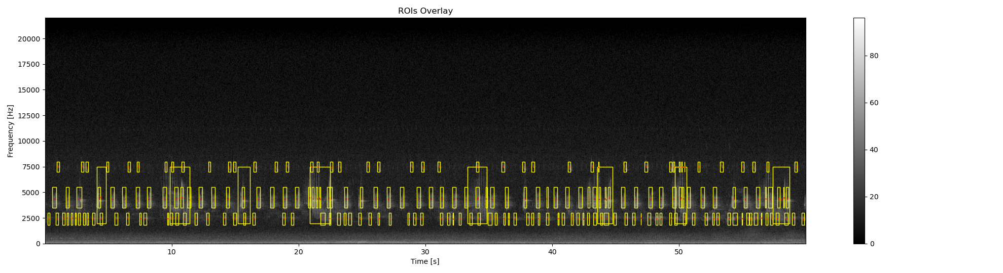
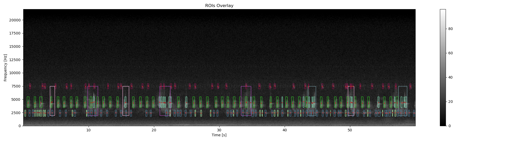
It is possible to extract Rois directly from the audio waveform without computing the spectrogram. This works well if there is no big overlap between each acoustic signature and you First, we have to define the frequency bandwidth where to find acoustic events In our example, there are clearly 3 frequency bandwidths (low : l, medium:m and high : h). We know that we have mostly short (ie. s) acoustic events in low, med and high frequency bandwidths but also a long (ie l) acoustic events in med. To extract

df_rois_sh = rois.find_rois_cwt(s, fs, flims=[7000, 8000], tlen=0.2, th=0.000001)
df_rois_sm = rois.find_rois_cwt(s, fs, flims=[3500, 5500], tlen=0.2, th=0.000001)
df_rois_lm = rois.find_rois_cwt(s, fs, flims=[2000, 7500], tlen=2,   th=0.0001)
df_rois_sl = rois.find_rois_cwt(s, fs, flims=[1800, 3000], tlen=0.2, th=0.000001)

## concat df
df_rois_WAV =pd.concat([df_rois_sh, df_rois_sm, df_rois_lm, df_rois_sl], ignore_index=True)

# drop rows with frequency and time outside of tn and fn
df_rois_WAV = df_rois_WAV[
   (df_rois_WAV.min_t >= tn.min()) &
   (df_rois_WAV.max_t <= tn.max()) &
   (df_rois_WAV.min_f >= fn.min()) &
   (df_rois_WAV.max_f <= fn.max())
   ]

# format dataframe df_rois_WAV in order to convert pixels into time and frequency
df_rois_WAV = format_features(
   df=df_rois_WAV,
   tn=tn,
   fn=fn
   )

# display rois
ax3, fig3 = overlay_rois(
   im_ref=Sxx_db,
   rois=df_rois_WAV,
   **{
      'vmin':0,
      'vmax':dB_max,
      'extent':ext
      }
   )

# get features: centroids
df_centroid_WAV = features.centroid_features(
   Sxx=Sxx_db,
   rois=df_rois_WAV
   )

# format dataframe df_centroid_WAV in order to convert pixels into time and frequency
df_centroid_WAV = format_features(
   df=df_centroid_WAV,
   tn=tn,
   fn=fn
   )

# display centroids
ax3, fig3 = overlay_centroid(
   im_ref=Sxx_db,
   centroid=df_centroid_WAV,
   savefig=None,
   **{'vmin':0,
      'vmax':dB_max,
      'extent':ext,
      'ms':2,
      'marker':'+',
      'color':'red',
      'fig':fig3,
      'ax':ax3
      }
   )

Prepare the features in order to have zero mean and same variance

X = StandardScaler().fit_transform(df_centroid_WAV[FEATURES])

# perform KMeans with the same number of clusters as with the manual annotation
labels = KMeans(
   n_clusters=NN_CLUSTERS,
   random_state=0,
   n_init='auto'
   ).fit_predict(X)

# Replace the unknow label by the cluster number predicted by KMeans
df_centroid_WAV['label'] = [str(i) for i in labels]

# overlay color bounding box corresponding to the label, and centroids
# on the original spectrogram
ax4, fig4 = overlay_rois(
   im_ref=Sxx_db,
   rois=df_centroid_WAV,
   **{
      'vmin':0,
      'vmax':dB_max,
      'extent':ext
      }
   )

ax4, fig4 = overlay_centroid(
   im_ref=Sxx_db,
   centroid=df_centroid_WAV,
   savefig=None,
   **{
      'vmin':0,
      'vmax':dB_max,
      'extent':ext,
      'ms':2,
      'fig':fig4,
      'ax':ax4
      }
   )

References

[1] Towsey, M., 2013b. Noise Removal from Wave-forms and Spectrograms Derived from Natural Recordings of the Environment. Queensland University of Technology, Brisbane