Simulation of sound degradation due to geometric, atmospheric and habitat attenuation

When sound travels in air (or in water), initial acoustic signature may change regarding distances due to attenuation. Sound attenuation in natural environment is very complex to model. We propose to reduce the complexity by decomposing the sound attenuation to three main sources of attenuation : - the geometric attenuation (Ageo) also known as spreading loss or geometric dispersion, - the atmospheric attenuation (Aatm) - and the habitat attenuation (Ahab). The later encompasses several sources of attenuation and might be seen as a proxy.

Load required modules

import matplotlib.pyplot as plt
from maad import sound, spl, util

Load the sound and conversion into sound pressure

When working with sound attenuation in real environment, it is essential to know the sound pressure level at a certain distance (generally 1m). Here we used spinetail sound. We assume that its sound level at 1m = 85dB SPL. It is also essential to be able to tranform the signal recorded by the recorder into sound pressure level. Here, the audio recorder is a SM4 (Wildlife Acoustics) which is an autonomous recording unit (ARU) from Wildlife. The sensitivity of the internal microphone is -35dBV and the maximal voltage converted by the analog to digital convertor (ADC) is 2Vpp (peak to peak). The gain used for the recording is a combination of the internal pre-amplifier of the SM4, which is 26dB and the adjustable gain which was 16dB. So the total gain applied to the signal is : 42dB

# We load the sound
w, fs = sound.load('../../data/spinetail.wav')
# We convert the sound into sound pressure level (Pa)
p0 = spl.wav2pressure(wave=w, gain=42, Vadc=2, sensitivity=-35)

Selection of the signal and the background noise

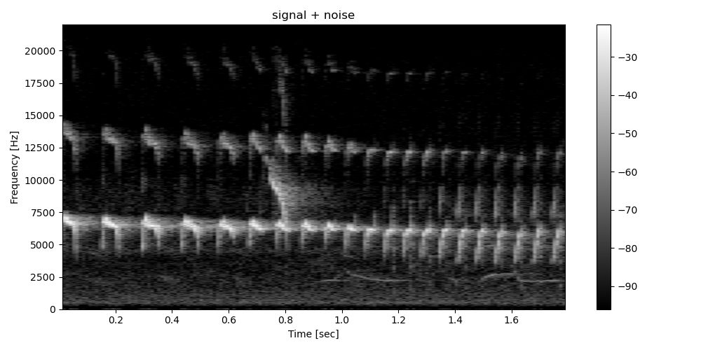
We select part of the sound with the spinetail signal

p0_sig = p0[int(5.68*fs):int(7.48*fs)]
# We select part of the sound with background
p0_noise = p0[int(8.32*fs):int(10.12*fs)]

We convert the spinetail signal into spectrogram

Sxx_power, tn, fn, ext = sound.spectrogram(p0_sig ,fs,
                                           display = True, figsize=[4,10], title = 'signal + noise')

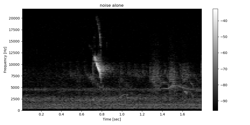
We convert the background signal into spectrogram

Sxx_power_noise, tn, fn, ext = sound.spectrogram(p0_noise ,fs,
                                                 display = True, figsize=[4,10], title = 'noise alone')

Then, we convert both spectrograms into dB. We choose a dB range of 96dB which is the maximal range for a 16 bits signal.

Sxx_dB = util.power2dB(Sxx_power, db_range=96) + 96
Sxx_dB_noise = util.power2dB(Sxx_power_noise, db_range=96) + 96

Evalution of the distance and sound level of the spinetail

Before simulating the attenuation of the acoustic signature depending on the distance, we need to evaluate the distance at which the signal of the spinetail was recordered. First, we estimate the sound level L of the spinetail song in the recording by selecting the sound between 6000-7000 Hz. We compute fast Leq (the equivalent sound level) within 100ms window and take the maximum Leq to be the estimated L of the call

F1 = 6000
F2 = 7000
p0_sig_bw= sound.select_bandwidth(p0_sig,
                                  fs,
                                  fcut=[F1,F2],
                                  forder=10,
                                  ftype='bandpass')
L =  max(spl.pressure2leq(p0_sig_bw, fs, dt=0.1))
print ('Sound Level measured : %2.2fdB SPL' %L)

Sound Level measured : 71.57dB SPL

Evalution of the distance between the ARU and the spinetail

Then, knowing the sound level L at the position of the ARU, we can estimate the maximum distance between the ARU and the position of the spinetail. This estimation takes into account the geometric, atmospheric and habitat attenuation (here, we use the default values to define atmospheric and habitat attenuation). This distance will be the reference distance r0

f,r0 = spl.detection_distance(L,
                              L0=85,
                              f=(F1+F2)/2)
print ('Max distance between ARU and spinetail is estimated to be %2.0fm' % r0)

Max distance between ARU and spinetail is estimated to be  4m

Evalution of the maximum distance of propagation of the spinetail song

Finally, we can estimate the detection distance or active distance of the spinetail which corresponds to the distance at which the call of the spinetail is below the noise level. First, we estimate the sound level of the background noise L_bkg_bw around the frequency bandwidth of the spinetail. We set background noise to min Leq. Then we estimate the average detection distance of the spinetail call (assuming that the initial level of the call @1m is 85dB SPL)

p0_noise_bw = sound.select_bandwidth(p0_noise,
                                     fs,
                                     fcut=[F1,F2],
                                     forder=10,
                                     ftype='bandpass')
L_bkg_bw = min(spl.pressure2leq(p0_noise_bw, fs, dt=0.1))
f, r = spl.detection_distance (L_bkg_bw,
                               L0=85,
                               f=(F1+F2)/2)
print('Max active distance is %2.1fm' %r)

Max active distance is 143.0m

Let’s see the contribution of each type of attenuation

_, df = spl.attenuation_dB (f=(F1+F2)/2,
                            r=r,
                            r0=1)

print(df)

        f      r    Ageo_dB   Aatm_dB  Ahab_dB    Asum_dB
0  6500.0  143.0  43.106721  8.604484    18.46  70.171204

Simulation of the attenuation of the acoustic signature at different distances

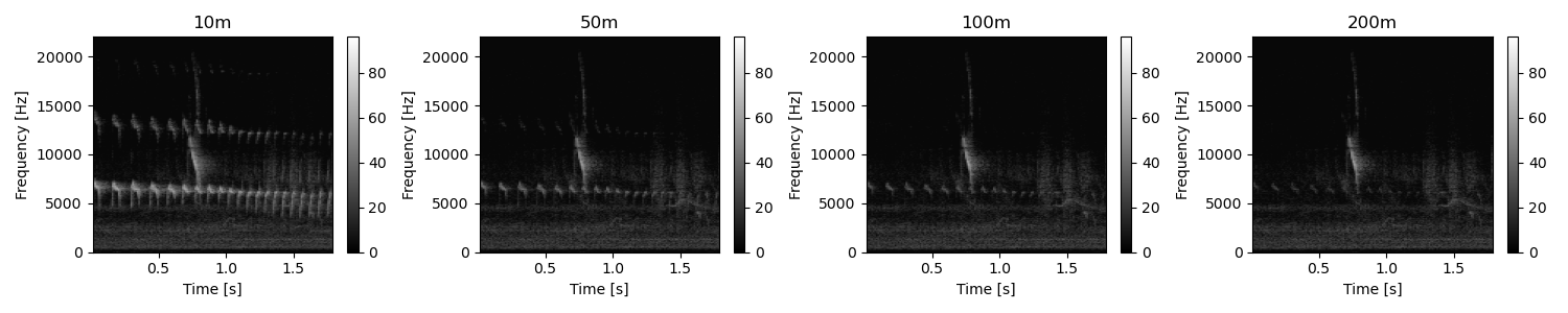
Knowing the distance r0 at which the signal was recorded from the source, we can simulate the attenuation of the acoustic signature depending on different distance of propagation. Here, we will simulate the attenuation of the signal after propagating 10m, 50m, 100m, 200m

Compute the attenuation of the recorded spinetail song at 10m.

p_att = spl.apply_attenuation(p0_sig, fs, r0 = r0, r = 10)
Sxx_power_att, tn, fn, ext = sound.spectrogram(p_att,fs)
Sxx_dB_att_10m = util.power2dB(Sxx_power_att,db_range=96) + 96

Compute the attenuation of the recorded spinetail song at 50m.

p_att = spl.apply_attenuation(p0_sig, fs, r0 = r0, r = 50)
Sxx_power_att, tn, fn, ext = sound.spectrogram(p_att,fs)
Sxx_dB_att_50m = util.power2dB(Sxx_power_att,db_range=96) + 96

Compute the attenuation of the recorded spinetail song at 100m.

p_att = spl.apply_attenuation(p0_sig, fs, r0 = r0, r = 100)
Sxx_power_att, tn, fn, ext = sound.spectrogram(p_att,fs)
Sxx_dB_att_100m = util.power2dB(Sxx_power_att,db_range=96) + 96

Compute the attenuation of the recorded spinetail song at 200m.

p_att = spl.apply_attenuation(p0_sig, fs, r0 = r0, r = 200)
Sxx_power_att, tn, fn, ext = sound.spectrogram(p_att,fs)
Sxx_dB_att_200m = util.power2dB(Sxx_power_att,db_range=96) + 96

Add noise to the signal. We add real noise recorded just after the song of the spinetail.

Sxx_dB_att_10m = util.add_dB(Sxx_dB_att_10m,Sxx_dB_noise)
Sxx_dB_att_50m = util.add_dB(Sxx_dB_att_50m,Sxx_dB_noise)
Sxx_dB_att_100m = util.add_dB(Sxx_dB_att_100m,Sxx_dB_noise)
Sxx_dB_att_200m = util.add_dB(Sxx_dB_att_200m,Sxx_dB_noise)

Plot attenuated spectrograms at different distances of propagation. We can observe that the highest frequency content (harmonics) disappears first. We can also observe that at 200m, almost none of the spinetail signal is still visible. Only the background noise, with the call of another species remains

fig, (ax1, ax2, ax3, ax4) = plt.subplots(1,4, sharex=True, figsize=(15,3))
util.plot2d(Sxx_dB_att_10m, title='10m',   ax=ax1, extent=ext, vmin=0, vmax=96, figsize=[3,3])
util.plot2d(Sxx_dB_att_50m, title='50m',   ax=ax2, extent=ext, vmin=0, vmax=96, figsize=[3,3])
util.plot2d(Sxx_dB_att_100m, title='100m', ax=ax3, extent=ext, vmin=0, vmax=96, figsize=[3,3])
util.plot2d(Sxx_dB_att_200m, title='200m', ax=ax4, extent=ext, vmin=0, vmax=96, figsize=[3,3])