Signal decomposition and false-color spectrograms

Soundscapes result from a combination of multiple signals that are mixed-down into a single time-series. Unmixing these signals can be regarded as an important preprocessing step for further analyses of individual components. Here, we will combine the robust characterization capabilities of the bidimensional wavelets [1] with an advanced signal decomposition tool, the non-negative-matrix factorization (NMF)[2]. NMF is a widely used tool to analyse high-dimensional data that automatically extracts sparse and meaningfull components of non-negative matrices. Audio spectrograms are in essence sparse and non-negative matrices, and hence well suited to be decomposed with NMF. This decomposition can be further used to generate false-color spectrograms to rapidly identify patterns in soundscapes and increase the interpretability of the signal [3]. This example shows how to use scikit-maad to easily decompose audio signals and visualize false-colour spectrograms.

Dependencies: This example requires the Python package scikit-learn v0.24 or greater.

# sphinx_gallery_thumbnail_path = './_images/sphx_glr_plot_nmf_and_false_color_spectrogram_003.png'

Load required modules

import numpy as np
import matplotlib.pyplot as plt
from maad import sound, features
from maad.util import power2dB, plot2d
from skimage import transform
from sklearn.preprocessing import MinMaxScaler
from sklearn.decomposition import NMF

Load audio from disk

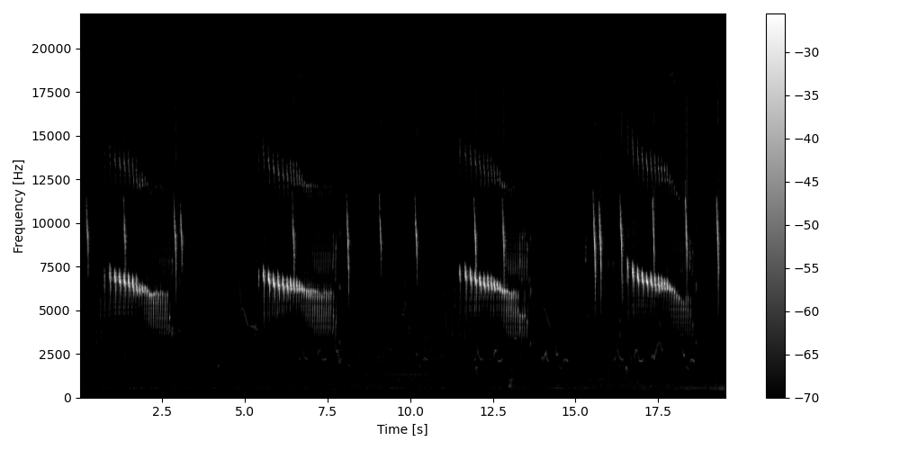
Load the audio file and compute the spectrogram.

s, fs = sound.load('../../data/spinetail.wav')
Sxx, tn, fn, ext = sound.spectrogram(s, fs, nperseg=1024, noverlap=512)

Sxx_db = power2dB(Sxx, db_range=70)
Sxx_db = transform.rescale(Sxx_db, 0.5, anti_aliasing=True, channel_axis=None)  # rescale for faster computation # multichannel=False change by  channel_axis=None
plot2d(Sxx_db, figsize=(4,10), extent=ext)

Filter the spectrogram with 2D wavelets

Compute feature with shape_features_raw to get the raw output of the spectrogram filtered by the filterbank composed of 2D Gabor wavelets. This raw output can be fed to the NMF algorithm to decompose the spectrogram into elementary basis spectrograms.

shape_im, params = features.shape_features_raw(Sxx_db, resolution='low')

# Format the output as an array for decomposition
X = np.array(shape_im).reshape([len(shape_im), Sxx_db.size]).transpose()

# Decompose signal using non-negative matrix factorization
Y = NMF(n_components=3, init='random', random_state=0).fit_transform(X)

Arrange into RGBA color model

Normalize the data and combine the three NMF basis spectrograms and the intensity spectrogram into a single array to fit the RGBA color model. RGBA stands for Red, Green, Blue and Alpha, where alpha indicates how opaque each pixel is.

Y = MinMaxScaler(feature_range=(0,1)).fit_transform(Y)
intensity = 1 - (Sxx_db - Sxx_db.min()) / (Sxx_db.max() - Sxx_db.min())
plt_data = Y.reshape([Sxx_db.shape[0], Sxx_db.shape[1], 3])
plt_data = np.dstack((plt_data, intensity))

Visualize output

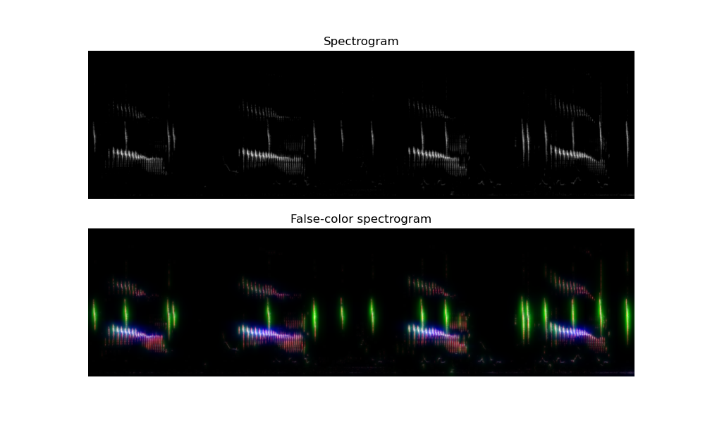
Finally, plot the resulting basis spectrogram as separate elements and combine them to produce a false-colour spectrogram using the RGBA color model.

fig, axes = plt.subplots(3,1, figsize=(10,8))
for idx, ax in enumerate(axes):
    ax.imshow(plt_data[:,:,idx], origin='lower', aspect='auto',
              interpolation='bilinear')
    ax.set_axis_off()
    ax.set_title('Basis ' + str(idx+1))

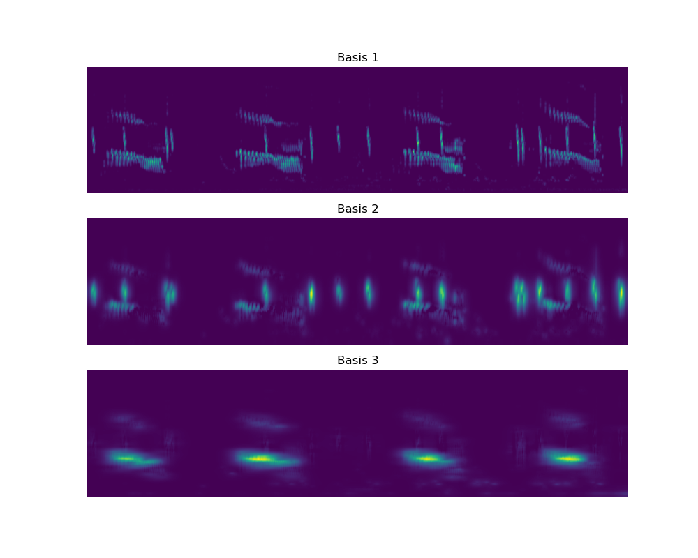
The first basis spectrogram shows fine and rapid modulations of the signal. Both signals have these features and hence both are delineated in this basis. The second basis highlights the short calls on the background, and the third component highlights the longer vocalizations of the spinetail. The three components can be mixed up to compose a false-colour spectrogram where it can be easily distinguished the different sound sources by color.

fig, ax = plt.subplots(2,1, figsize=(10,6))
ax[0].imshow(Sxx_db, origin='lower', aspect='auto', interpolation='bilinear', cmap='gray')
ax[0].set_axis_off()
ax[0].set_title('Spectrogram')
ax[1].imshow(plt_data, origin='lower', aspect='auto', interpolation='bilinear')
ax[1].set_axis_off()
ax[1].set_title('False-color spectrogram')

References

[1] Sifre, L., & Mallat, S. (2013). Rotation, scaling and deformation invariant scattering for texture discrimination. Computer Vision and Pattern Recognition (CVPR), 2013 IEEE Conference On, 1233–1240. http://ieeexplore.ieee.org/xpls/abs_all.jsp?arnumber=6619007

[2] Lee, D., & Sueng, S. (1999). Learning the parts of objects by non-negative matrix factorization. Nature, 401, 788–791. https://doi.org/10.1038/44565

[3] Towsey, M., Znidersic, E., Broken-Brow, J., Indraswari, K., Watson, D. M., Phillips, Y., Truskinger, A., & Roe, P. (2018). Long-duration, false-colour spectrograms for detecting species in large audio data-sets. Journal of Ecoacoustics, 2(1), 1–1. https://doi.org/10.22261/JEA.IUSWUI